GPS Estimation

One major component of the Nebula project is its GPS Estimation module. In our GitHub repository, it is located under the src/controls/detection directory. This module is responsible for estimating the GPS coordinates of a single pixel within a camera frame captured by a nadir (downward-facing) mounted camera.

The GPS Estimation module is designed for a monocular camera setup, meaning it uses a single camera to capture images and estimate GPS coordinates. This contrasts with stereo camera setups, which use two cameras to obtain depth information. Our implementation is based on the pinhole camera model.

In essence, the GPS Estimation module consists of two main parts:

Object localization - estimating the exact pixel location of the target object (e.g., helipad or tank) within the camera frame using our image recognition model.
Coordinate estimation - computing the GPS coordinates of that pixel using the camera’s intrinsic and extrinsic parameters, along with the drone’s GPS position and altitude provided via MAVLink.

Image Recognition

Our Image Recognition model is a custom-trained YOLOv8 model. It is trained to detect four classes of objects: helipad, tank, sim_helipad, and sim_tank — representing two sets of real and simulated objects (helipad and tank).

The sim_helipad class is a subset of helipad-tagged images collected exclusively from the simulated environment. Similarly, sim_tank is a subset of tank-tagged images captured from simulations.

We trained our model on nearly a thousand images combined from both real-world and simulated environments. The model is designed to detect these objects not only from a nadir (downward-facing) camera view but also from various oblique angles.

For image annotation, we used the Roboflow platform. After annotating the dataset, we exported it in YOLO format and trained the model using Google Colab. The overall process is straightforward, though somewhat time-consuming.

Note

At times pytorch for running this weight might be mismatched. Please ensure you have the correct version of pytorch installed. To verify that run the command:

make test_torch

Camera Calibration

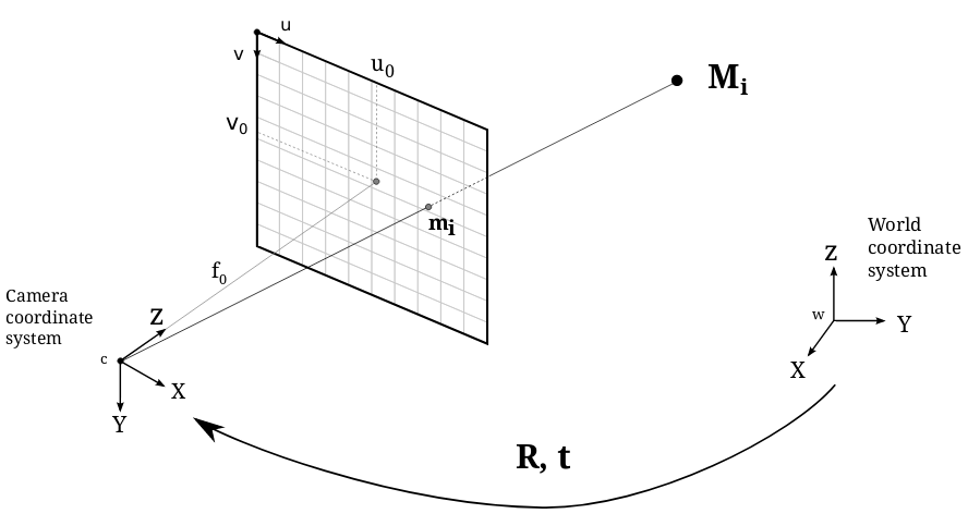
To estimate GPS coordinates from pixel locations, we first need to know the camera’s intrinsic parameters. These include the focal length, principal point, and distortion coefficients.

Using these intrinsic parameters, we apply the pinhole camera model to map 3D world coordinates to 2D image coordinates. This mapping can then be reversed to project 2D image coordinates back into 3D world space — a standard computer vision technique.

For calibration, we use OpenCV’s chessboard calibration method. You can follow this tutorial for a detailed guide on camera calibration using OpenCV,

or use our implementation available at controls/detection/camera_calibration.py within the repository.

While some pinhole cameras introduce significant distortion, primarily radial and tangential distortion, our setup uses a high-quality camera with a wide-angle lens that produces minimal distortion. Therefore, we can safely ignore distortion coefficients in our calculations.

In practice, we primarily use the focal length and principal point for GPS estimation. However, it is generally more accurate to use the complete camera intrinsic matrix (K matrix) obtained from the calibration process.

GPS Coordinate Estimation

Once we have the pixel coordinates of the object of interest from our image recognition model and the camera’s intrinsic parameters from the calibration process, we can proceed to estimate its GPS coordinates.

The GPS estimation process involves several ordered steps, summarized below. We assume a nadir-mounted camera (with the optical axis approximately aligned downward) and negligible lens distortion — either ignored or compensated for during preprocessing.

The procedure is presented in a clear, step-by-step manner, followed by the key mathematical formulas used in the computation.

Steps

Get drone reference: obtain the drone’s current GPS coordinates (latitude \(\phi_0\), longitude \(\lambda_0\)) and altitude \(h\) above the ellipsoid (or above ground if available). For higher accuracy use RTK-corrected GPS instead of raw GNSS data.
Get camera pose: obtain the camera extrinsics relative to the drone body and the drone attitude (rotation/roll/pitch/yaw). From these we build the rotation \(R_{cb}\) (camera-to-body) and \(R_{be}\) (body-to-ENU/world) matrices. Combined camera-to-ENU rotation is \(R_{ce} = R_{be} \; R_{cb}\).
Convert pixel to normalized camera coordinates (back-projection): using the intrinsic matrix K, map pixel (u, v) to a ray in camera coordinates.

\[\begin{split}K = \begin{bmatrix} f_x & 0 & c_x \\ 0 & f_y & c_y \\ 0 & 0 & 1 \end{bmatrix}\end{split}\]

Given pixel coordinates \((u, v)\) and homogeneous form \(\tilde{p} = [u, v, 1]^T\), the normalized camera ray (direction) is

\[\begin{split}r_c = K^{-1} \tilde{p} = \begin{bmatrix} x_c \\ y_c \\ 1 \end{bmatrix} ,\end{split}\]

where \(x_c = (u - c_x)/f_x\) and \(y_c = (v - c_y)/f_y\) for a pinhole model with no skew.
Rotate ray into ENU/world frame: using the camera-to-ENU rotation \(R_{ce}\), obtain the ray in ENU coordinates

\[r_e = R_{ce} \; r_c\]

The camera origin in ENU coordinates is the drone position at altitude \(h\): \(p_e = [0, 0, h]^T\) if we place ENU origin at the drone’s ground-projected location, or use the true ENU coordinates computed from \(\phi_0, \lambda_0, h_0\).
Intersect ray with ground plane (approximate flat Earth locally): assume ground is at altitude \(z = 0\) in ENU frame (or at known ground elevation). Parametric ray from camera origin:

\[p_e(t) = p_{cam} + t \; r_e, \qquad t > 0\]

Solve for t such that the z-component equals ground altitude z_g (typically 0):

\[t^* = \frac{z_g - p_{cam,z}}{r_{e,z}}\]

Then the intersection point in ENU is

\[P_{enu} = p_{cam} + t^* \; r_e\]

Note: if \(r_{e,z} \approx 0\) (ray nearly parallel to ground) the intersection is unstable; handle this edge case by rejecting or using a different method (e.g., local DEM).
Convert ENU coordinates to geodetic coordinates (latitude, longitude): given ENU offset \(\Delta E = [e, n, u]^T\) from reference geodetic point \((\phi_0, \lambda_0, h_0)\), convert back to latitude/longitude. For small distances you can use the local flat-earth approximation:

\[\Delta \phi \approx \frac{n}{R_N + h_0}, \qquad \Delta \lambda \approx \frac{e}{(R_E + h_0) \cos\phi_0}\]

where \(R_N\) and \(R_E\) are radii of curvature (or simply use Earth’s mean radius R approx 6371000 m for small offsets). Then

\[\phi = \phi_0 + \Delta \phi, \qquad \lambda = \lambda_0 + \Delta \lambda\]
Output estimated GPS coordinates (latitude, longitude) and optionally estimated horizontal uncertainty derived from altitude and detection pixel uncertainty.

Extra Considerations if Needed

If you want to improve accuracy or handle edge cases, consider the following:

Distortion: If distortion is not negligible, undistort the pixel coordinates before performing back-projection using the distortion coefficients obtained during calibration.
Altitude reference: Ensure that the altitude values used for the camera origin and ground plane (\(z_g\)) share the same vertical datum (e.g., above ellipsoid, above mean sea level, or above ground level). Mismatched altitude references can introduce significant bias in the estimated GPS coordinates.
Attitude accuracy: Even small errors in pitch or roll can lead to large horizontal errors, especially at higher altitudes. Quantify and account for these uncertainties accordingly.
Near-parallel rays: When the back-projected ray is nearly parallel to the ground (\(r_{e,z} \approx 0\)), the ground intersection becomes numerically unstable. In such cases, either reject the estimate or use a Digital Elevation Model (DEM) or optical flow-based scale estimation to improve stability.